Quantifying Swiss Cheese, the Bayesian Way

Quantifying Swiss Cheese, the Bayesian Way

Author’s Note

This article is part of my research exploring quantitative methods for vulnerability risk management and exploit likelihood modeling. If you haven’t yet, you should start with the first piece, Modeling Asset Risk Using EPSS, where I introduce the foundation for this approach.

The views presented in this blog are entirely my own and do not represent the views of any organization or other affiliation.

This piece demonstrates a framework using synthetic data to illustrate the concept. Focus on the method, not the numbers.

Last year, I explored how to estimate asset-level exploit likelihood using EPSSg — the probability that at least one vulnerability on an asset will be exploited in the wild based on EPSS data. That model helped visualize which assets experience the highest external exploit pressure and prioritize defensive actions accordingly. I presented this at VulnCon 2025.

However, this view was limited and made one major assumption: it assumed all of your assets were equally likely to be targeted without compensating controls in place. That model was useful as a starting point, though it assumed all assets were equally exposed — an assumption we know is false.

In reality, we have layers of defenses — from patching timelines to intrusion prevention systems at the network and endpoint layer. These layers reduce the probability that exploits actually succeed. So in order to iterate the model, we can use Bayesian inference to incorporate control effectiveness rates for controls that prevent exploit attempts. The question becomes: how do we translate those layers into measurable probabilities?

In this follow-up, I’ll show you how to incorporate control effectiveness into EPSSg to try to answer the question:

What is the exploitation likelihood of at least one (1) vulnerability on this asset, given the controls in place?

Recap: EPSS and EPSSg

The Exploit Prediction Scoring System (EPSS) is a machine-learning model that publishes the likelihood of a CVE being exploited within the next thirty (30) days. Each CVE gets a likelihood value between 0 and 1 — the higher the score, the greater the chance of exploitation.

EPSSg (or Grouped EPSS) is the probability that at least one (1) vulnerability on a given asset will see exploitation activity in the next thirty (30) days. We calculate it using the classic “at least one” formula from probability theory. If each CVE i has probability EPSSi, then the probability that none are exploited is the product of their non-exploitation probabilities (the inverse of the EPSS score). Subtracting from 1 gives us the probability of at least one i CVE, which I call EPSSg:

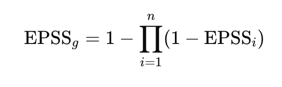
This provides a baseline probability of exploitation for each asset — assuming no controls. It’s a “worst-case exposure” measure. So how do we factor in our security controls?

Quantifying Swiss Cheese

Swiss Cheese Model

Think of your organization’s defenses as layers of Swiss cheese. Each layer has some holes (no control is 100% effective), but multiple layers together can reduce the chance of an attacker slipping through all of them. This is the classic Swiss cheese model of risk management. If the holes (control failures) don’t line up, the threat is stopped; only when all holes align does the bad outcome occur.

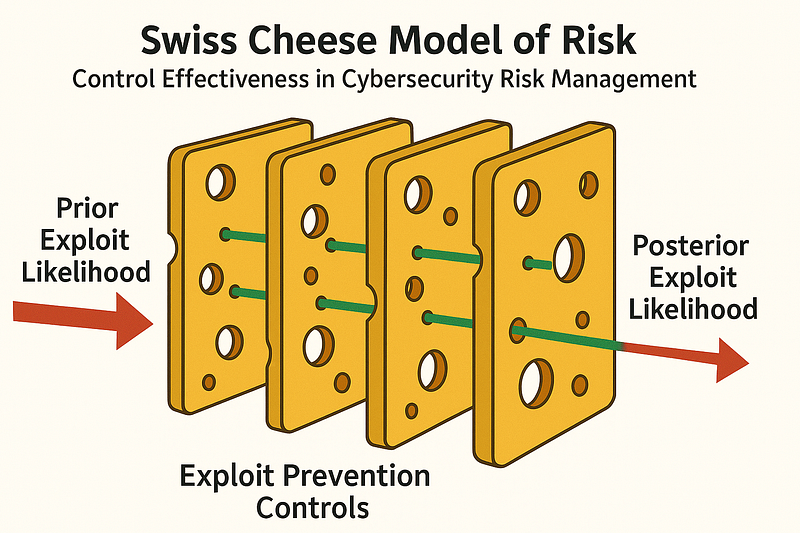
This is where Bayesian inference enters the picture. Applying this to exploit likelihood means we can treat each control as a probabilistic filter that reduces the base exploitation likelihood from EPSSg. To do this rigorously, we need a way to quantify how effective each layer is — and to update that belief over time.

Caveats and assumptions

No model mirrors reality perfectly — but building a quantifiable starting point lets us iteratively align our assumptions with new evidence.

Let’s dive into a few assumptions we need to establish.

1. EPSS is representative of global exploitation pressure, a proxy for attacker behavior across the internet
2. Vulnerabilities with a CVE are not the only vulnerabilities in our software. EPSS covers only CVE-tagged vulnerabilities, a large but incomplete subset of all flaws. Still, it’s the only publicly available probabilistic dataset, making it the most practical foundation.
3. Grouped EPSS (EPSSg) is the public exploit pressure on this asset if it were on the public internet.
4. Control Effectiveness rates assume that given the population of vulnerabilities, the control prevents exploitation X% of the time. Controls are treated as independent layers — an assumption we can later test with telemetry.

With those assumptions set, we can start quantifying how much each defensive slice of cheese actually helps.

Modeling Control Effectiveness

In this context, I define control effectiveness as the probability that a given control prevents the exploitation of a vulnerability. Think of it as the defensive success rate for a specific layer.

For example:

• A network firewall might block 70% of exploit attempts.
• An EDR might stop 60%.
• Assuming their effects are roughly independent, combined coverage could push actual likelihood well below the baseline.

But how do we know those percentages?

We usually don’t. Vendor claims are vague, telemetry can be incomplete, and empirical data is scarce. So we start with informed estimates — structured, measurable beliefs we can later update with data.

SME Beliefs

One practical way to form our initial belief (the prior) is to survey subject matter experts (SMEs) about control performance. Even if imperfect, this exercise builds a culture of quantitative reasoning and provides the starting point for Bayesian updating.

That notion aside, we can construct a survey question using a scenario that accounts for our assumptions:

Given an asset with 10 vulnerabilities present behind a well-configured firewall, how many does the firewall prevent the exploitation of?

In this context, we can define well-configured as one that meets our internal standards (e.g., signatures current, traffic monitored, rule sets tuned).

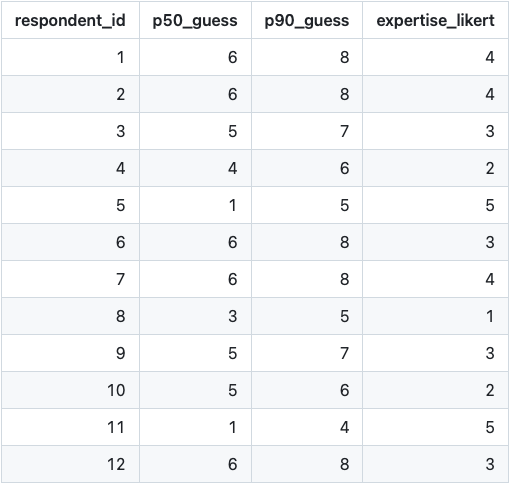
The answer options are integers between 0 and 10. Drawing on inspiration from How to Measure Anything in Cybersecurity Risk (Hubbard & Seiersen) and The Metrics Manifesto (Seiersen), we ask twice: once for the median estimate (we directly ask our SMEs for an answer to the question and assume it’s the median value), and again for the 90th-percentile value — the number they’re 90% confident the true effectiveness is below.

We then weight responses by self-rated expertise on a Likert scale (1 = novice, 5 = expert), producing both equal-weight and expertise-weighted models.

Sample responses

Let’s say for demonstration purposes that we survey 12 SMEs. An example of those responses is below:

Beliefs to Beta

In order to analyze this data, we turn to the Beta distribution. The Beta distribution is ideal for representing probabilities between 0 and 1 when we have uncertainty. The Beta distribution accepts two parameters:

• α (alpha) which is equal to the number of successes + 1
• β (beta) which is equal to failures + 1

In simple terms, α and β shape the curve describing how confident we are about control success and failure rates.

Our challenge is to infer α and β from SME p50 and p90 values. In Python, we can use fsolve from scipy.optimize to reverse-engineer the Beta parameters that produce those percentiles.

from scipy.stats import beta
from scipy.optimize import fsolve

def solve_alpha_beta(p50, p90):
    def equations(params):
        a, b = params
        return (
            beta.cdf(p50, a, b) - 0.5,  # p50 target
            beta.cdf(p90, a, b) - 0.9   # p90 target
        )
    return fsolve(equations, (2, 5))  # initial guess for α and β

This function finds α and β whose cumulative distribution matches our SME-reported medians and 90th percentiles. By running this across all SME responses, we can build aggregate Beta distributions — both equally weighted and expertise-weighted versions — to visualize our shared belief about the control’s effectiveness and show the shape of our uncertainty.

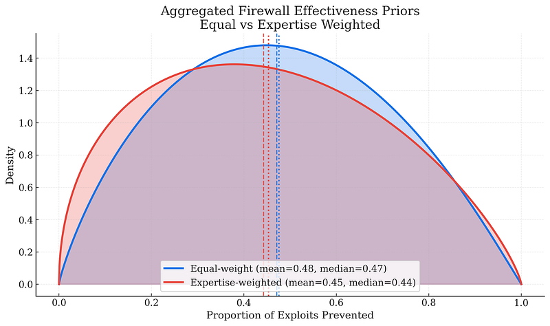
These distributions give us multiple values to pick for our central tendency single point value. In this scenario, I usually pick the lowest value in order to remain conservative with our judgments and overstate risk. Based on our example here, I would select a firewall control effectiveness rate for exploit prevention of 0.44, the expertise-weighted median value. The wide spread reminds us that uncertainty remains high until we gather more data.

Updating our Beliefs: The Bayesian Way

Integrating Control Effectiveness with EPSSg

Once we have a control effectiveness rate, we can update our asset-level exploit likelihood by multiplying it by the inverse of our control effectiveness rate (our control failure rate).

If an asset’s EPSSg is 0.76 and our firewall effectiveness posterior mean is 0.44, then:

That’s a 42% adjusted exploit likelihood — more realistic than assuming total exposure.

Continuously Updating Control Effectiveness

Now that we have our initial beliefs quantified, we can now update them with observations. Observation data can come in many forms, and for the firewall effectiveness example, we can likely look at our firewall logs to find exploit-related events. We could formulate a system that parses these logs and picks out the events that were successes and failures, depending on what type of logic an organization wants to implement.

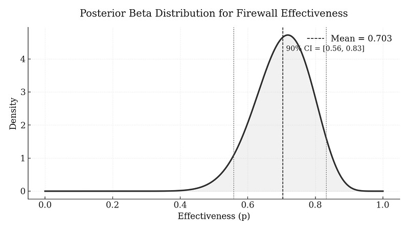
For our example here, let’s say we observe 15 successful exploit prevention events from our firewall logs, and 5 unsuccessful events in the next month. Using the reverse-engineered alpha and beta values from our expertise-weighted Beta distribution, we update our beliefs like so:

Below is the resulting Beta distribution. The central tendency (our updated best estimate of control effectiveness) increased from 0.44 to 0.703, meaning we’ve gained confidence that the firewall blocks about 70.3% of exploit attempts. Our confidence interval also tightened.

We can then turn around and make yet another update to our exploit likelihood on the asset (In practice, EPSS updates daily, so the asset’s baseline likelihood will shift as well.):

From Static to Living Models

This process transforms our exploit likelihood model into a living system that evolves as evidence accumulates. Observation sources include:

• Firewall and EDR telemetry — blocked vs. successful exploit attempts
• Breach and attack simulation tools like Picus Security¹
• Red team or purple team exercises
• Incident reports tied to control failures
• Any feedback loop that distinguishes success from failure can feed the model

Each update shifts our posterior a little closer to reality. Over time, our understanding of “how holey our cheese really is” becomes quantifiable.

So what?

A shared, continuously updated model lets all stakeholders align on reality and make smarter decisions about time, effort, and budget.

In vulnerability management, our goal is to reduce exploit risk. By quantifying control effectiveness transparently, we strengthen trust in both the model and the decisions it supports.

Future Considerations

FAIR-CAM

If you’re familiar with FAIR-CAM (Factor Analysis of Information Risk — Controls Analytics Model), you’ll recognize the conceptual overlap. FAIR-CAM formalizes how individual control functions combine to influence overall loss event frequency.

I view what I outline here as FAIR-CAM lite — a focused, quantitative slice of that same principle, applied specifically to exploit prevention. Instead of modeling every control family, we’re zooming in on how a single control’s effectiveness updates our belief in exploit likelihood through Bayesian inference. It’s a practical on-ramp for teams not yet ready for full FAIR-CAM implementation.

The structure is identical in spirit:

• EPSSg represents threat event frequency (global exploit pressure).
• Control effectiveness functions as resistance strength (how often the control stops that pressure).
• Bayesian updating mirrors FAIR-CAM’s goal of adjusting control factors as evidence accumulates.

In other words, this framework is an applied subset of FAIR-CAM — one that demonstrates how you can begin quantifying and updating control performance today, even before a full FAIR-CAM implementation.

Multiple Controls

What I demonstrated here was the use of a single control’s effectiveness in reducing exploitation likelihood. However, organizations usually have multiple controls in place, and FAIR-CAM accounts for this. We can borrow that logic and apply it directly to this scenario by building additional control effectiveness models to update the exploit likelihood in succession:

Exploit Vector Incident Likelihood

What if we could model the likelihood of an incident that includes exploitation within our environment? Where would we start, and how could we continuously update this model with observations? These questions point toward a vulnerability-to-incident pipeline, a frontier I am currently exploring.

Wrapping Up

We can’t eliminate uncertainty — but we can measure it, update it, and communicate it.

Bayesian updating gives us a disciplined way to evolve our beliefs as evidence accumulates. By pairing EPSSg (our view of global exploit pressure) with quantified control effectiveness, we move from static assumptions to a dynamic, evidence-driven model.

Each layer of Swiss cheese becomes a measurable probability curve — not just a metaphor, but a quantifiable defense system we can track, test, and improve.

1. Disclosure: I am a paid advisor for Picus Security, but Picus did not sponsor or influence this methodology.

Have more questions about EPSS? Check out the FAQ here, or join the EPSS Special Interest Group (SIG) to engage directly with the chairs and other vulnerability management, risk modeling, and data science enthusiasts.